How a Distributed Plan is Built#

This page walks through how the distributed DataFusion planner transforms a query into a distributed execution plan.

The transformation runs as a DataFusion QueryPlanner (registered by with_distributed_planner()) after normal physical planning. It takes the single-node physical plan, finds the points where data would cross a thread boundary in vanilla DataFusion, and inserts a network boundary node there instead — splitting the plan into stages that run on different tasks (machines).

The same plan, before and after#

Take SELECT count(*), "RainToday" FROM weather GROUP BY "RainToday" ORDER BY count(*) over a 3-file table on a 3-worker cluster. Here is the ordinary single-node physical plan (file paths trimmed to [...]):

SortPreservingMergeExec: [count(*)@0 ASC NULLS LAST]
  SortExec: expr=[count(*)@0 ASC NULLS LAST], preserve_partitioning=[true]
    ProjectionExec: expr=[count(Int64(1))@1 as count(*), RainToday@0 as RainToday]
      AggregateExec: mode=FinalPartitioned, gby=[RainToday@0 as RainToday], aggr=[count(Int64(1))]
        RepartitionExec: partitioning=Hash([RainToday@0], 4), input_partitions=3
          AggregateExec: mode=Partial, gby=[RainToday@0 as RainToday], aggr=[count(Int64(1))]
            DataSourceExec: file_groups={3 groups: [...]}, projection=[RainToday], file_type=parquet

And the distributed plan for the same query, rendered with display_plan_ascii:

┌───── DistributedExec ── Tasks: t0:[p0]
│ SortPreservingMergeExec: [count(*)@0 ASC NULLS LAST]
│   [Stage 2] => NetworkCoalesceExec: output_partitions=8, input_tasks=2
└──────────────────────────────────────────────────
  ┌───── Stage 2 ── Tasks: t0:[p0..p3] t1:[p0..p3]
  │ SortExec: expr=[count(*)@0 ASC NULLS LAST], preserve_partitioning=[true]
  │   ProjectionExec: expr=[count(Int64(1))@1 as count(*), RainToday@0 as RainToday]
  │     AggregateExec: mode=FinalPartitioned, gby=[RainToday@0 as RainToday], aggr=[count(Int64(1))]
  │       [Stage 1] => NetworkShuffleExec: output_partitions=4, input_tasks=3
  └──────────────────────────────────────────────────
    ┌───── Stage 1 ── Tasks: t0:[p0..p7] t1:[p0..p7] t2:[p0..p7]
    │ RepartitionExec: partitioning=Hash([RainToday@0], 8), input_partitions=3
    │   AggregateExec: mode=Partial, gby=[RainToday@0 as RainToday], aggr=[count(Int64(1))]
    │     DistributedLeafExec: DataSourceExec: file_groups={3 groups: [...]}, projection=[RainToday], file_type=parquet
    └──────────────────────────────────────────────────

Same operators, same order. The planner only:

inserted a NetworkShuffleExec above the hash RepartitionExec (the shuffle now fans data across tasks),
inserted a NetworkCoalesceExec at the top to gather all tasks into the single head task,
wrapped the leaf in a DistributedLeafExec so each task scans its own slice of the files, and
grew the shuffle’s partition count (4 → 8) because it now feeds multiple tasks.

Reading the output#

┌───── Stage 1 ── Tasks: t0:[p0..p7] t1:[p0..p7] t2:[p0..p7] — a stage running on 3 tasks (t0, t1, t2), each on a different worker, each executing partitions p0..p7. Tasks are machines; partitions are the threads within a task.
[Stage 1] => NetworkShuffleExec: output_partitions=4, input_tasks=3 — a network boundary: this node streams the output of Stage 1 over Arrow Flight instead of from a child node. input_tasks is how many tasks produced the data; output_partitions is how many partitions it exposes to its parent.
DistributedExec — the root and the only node the client executes. It hosts the head stage, which always runs on a single task (the coordinator).
DistributedLeafExec — a transparent wrapper around the original leaf; DistributedExec swaps in the right per-task variant before sending the stage to a worker.

Step by step#

The rest of this page walks the same transformation visually, on a four-file aggregation. To better understand what happens with the plan in the distribution process, we will represent it graphically:

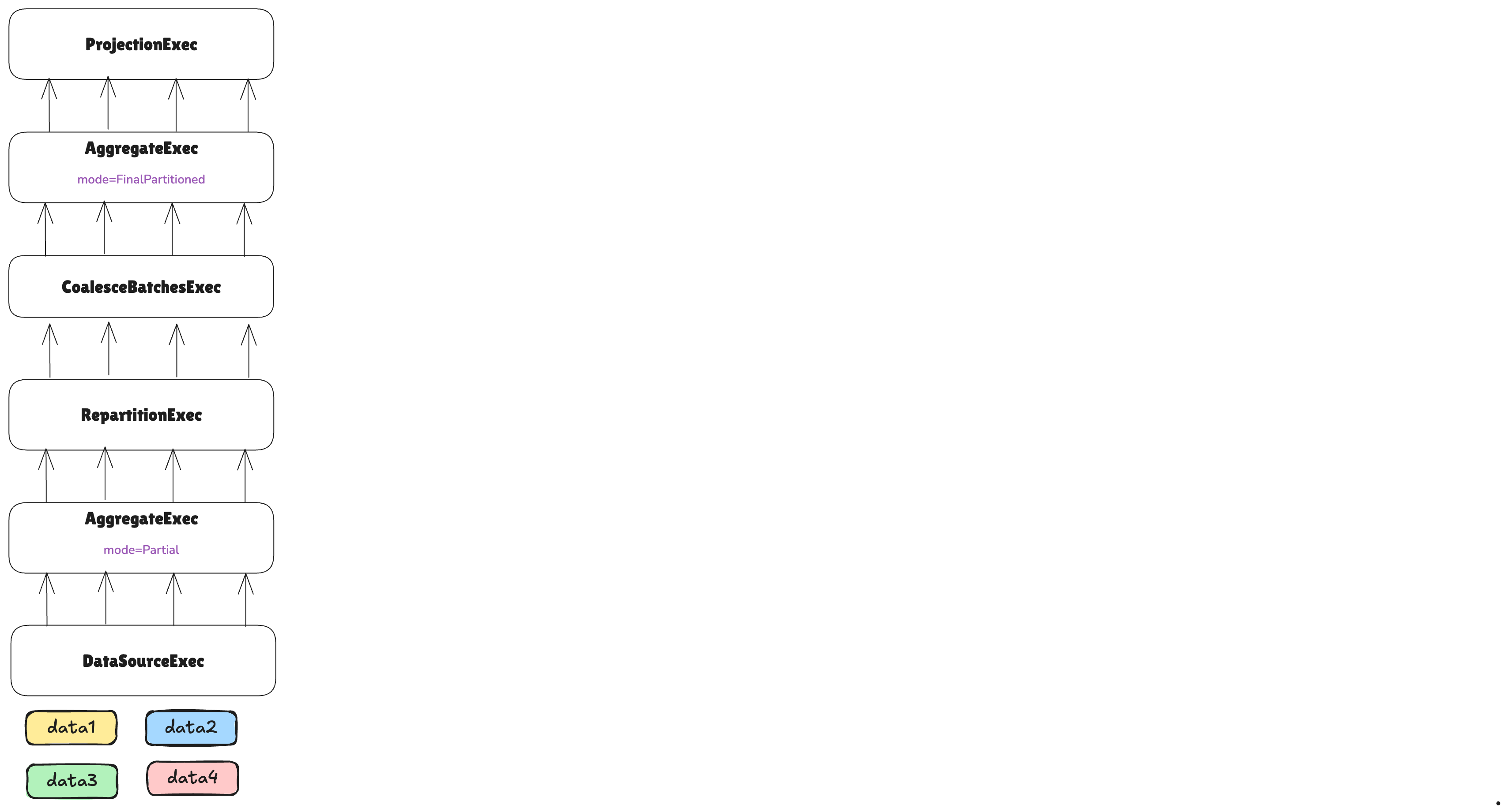
Note how the underlying DataSourceExec contains multiple non-overlapping pieces of data, represented with colors in the image. Depending on the underlying DataSource implementation in the DataSourceExec node, these can represent different things, such as different parquet files, or an external API from which we can gather data for different time ranges.

The first step is to split the leaf node into different tasks:

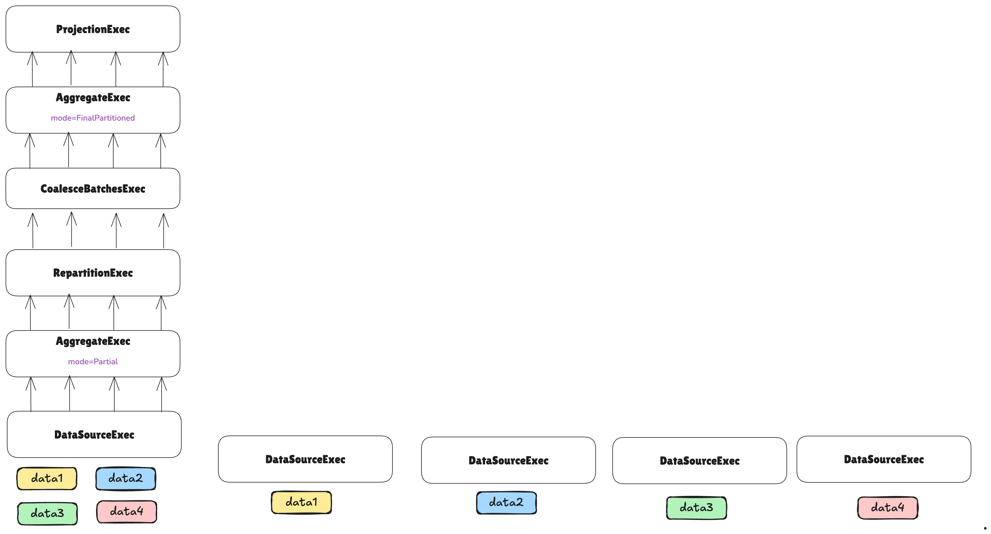
Each task will handle a different non-overlapping piece of data.

The number of tasks that will be used for executing leaf nodes is determined by a TaskEstimator implementation. A default implementation exists for file-based DataSourceExec nodes. However, since DataSourceExec can be customized to represent any data source, users with custom implementations should also provide a corresponding TaskEstimator.

In the case above, a TaskEstimator decided to use four tasks for the leaf node. Note that even if we are distributing the data across different tasks, each task will also distribute its data across partitions using the vanilla DataFusion partitioning mechanism. A partition is a split of data processed by a single thread on a single machine, whereas a task is a split of data processed by an entire machine within a cluster.

After that, we can continue reconstructing the plan:

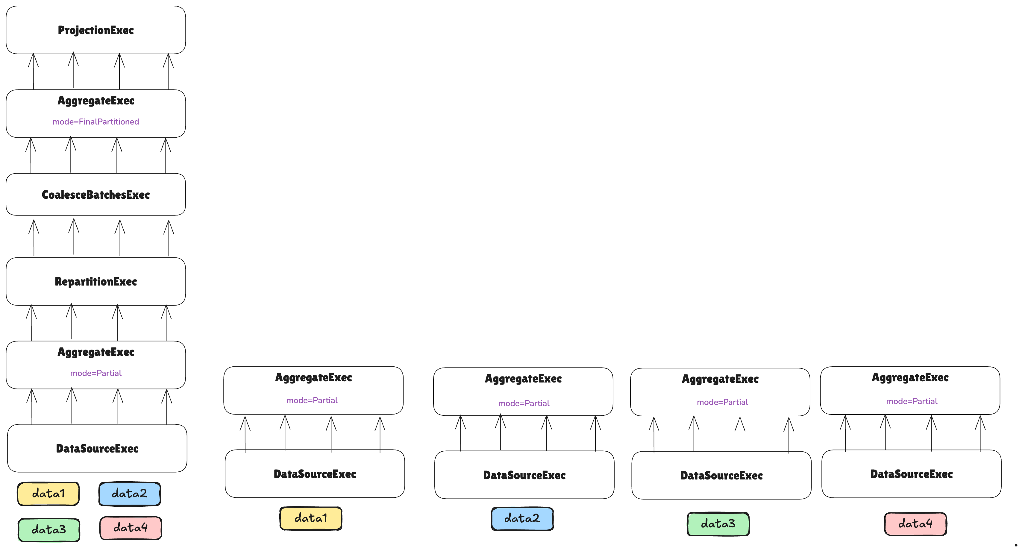
Nothing special to consider for now—the partial aggregation can simply be executed in parallel across different workers without further considerations.

Let’s keep constructing the plan:

At this point, the plan encounters a RepartitionExec node, which requires repartitioning data so each partition handles a non-overlapping subset of grouping keys for the aggregation.

While RepartitionExec redistributes data across threads on a single machine in vanilla DataFusion, it redistributes data across threads on different machines in the distributed context—requiring a network shuffle.

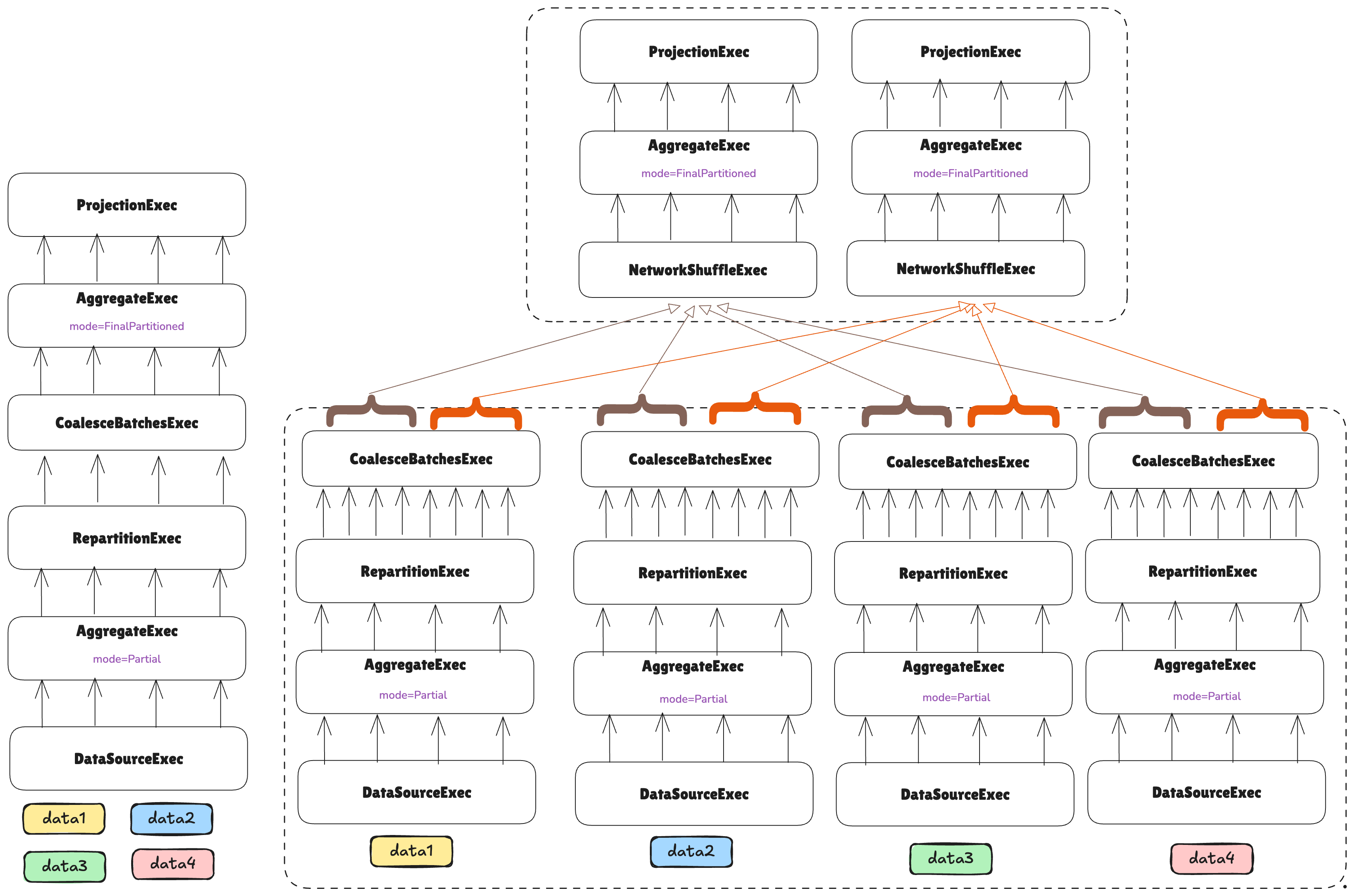
As we are about to send data over the network, it’s convenient to coalesce smaller batches into larger ones to avoid the overhead of sending many small messages, and instead send fewer but larger messages:

After this, we are ready to perform the shuffle over the network. For that, a new ExecutionPlan implementation is provided: NetworkShuffleExec:

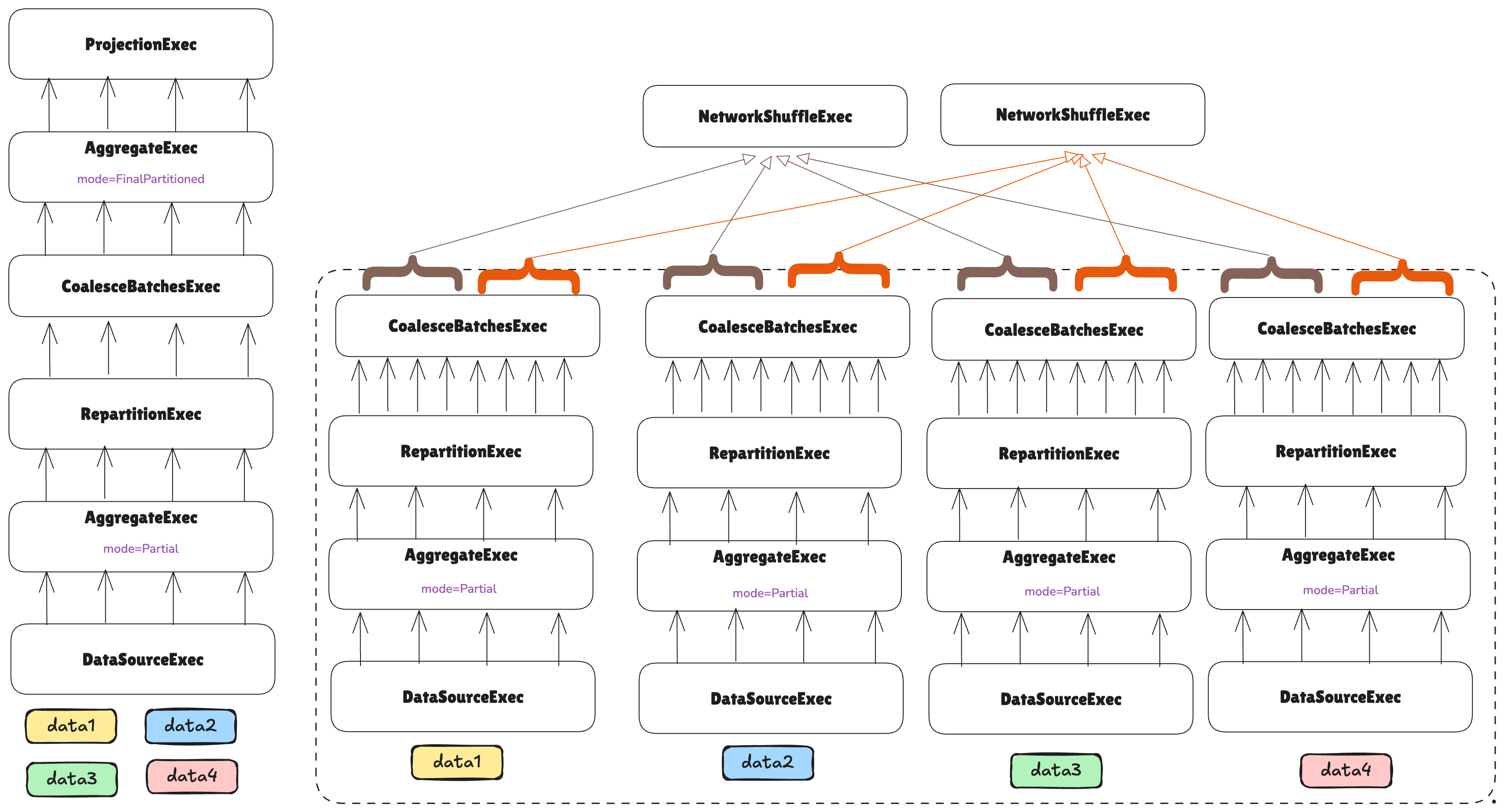
A NetworkShuffleExec, instead of calling execute() on its child node, will execute it remotely through Arrow Flight, and each NetworkShuffleExec instance will know from which partitions and machines it should gather data.

Note how this means that we have just built the first stage, as the first network boundary was introduced. We are now in the process of building the second stage, and note how it has just two tasks.

If the number of tasks in a leaf stage is driven by the hints given by TaskEstimators, the number of tasks in upper stages is driven by the nodes in between that reduce or increase the cardinality of the data.

In this case, the leaf stage is performing a partial aggregation before sending data to the next stage, so we can assume that less compute will be needed, and therefore, we can reduce the width of the next stage to just two tasks.

The rest of the plan can be formed as normal:

One final step remains: the plan’s head is currently distributed across two machines, but the final result must be consolidated on a single node. In the same way that vanilla DataFusion coalesces all partitions into one in the head node for the user, we also need to do that, but not only across partitions on a single machine, but across tasks on different machines.

For that, the NetworkCoalesceExec network boundary is introduced: it coalesces P partitions across N tasks into N*P partitions in one task. This does not imply repartitioning, or shuffling, or anything like that. The partitions are the same but joined into a single task:

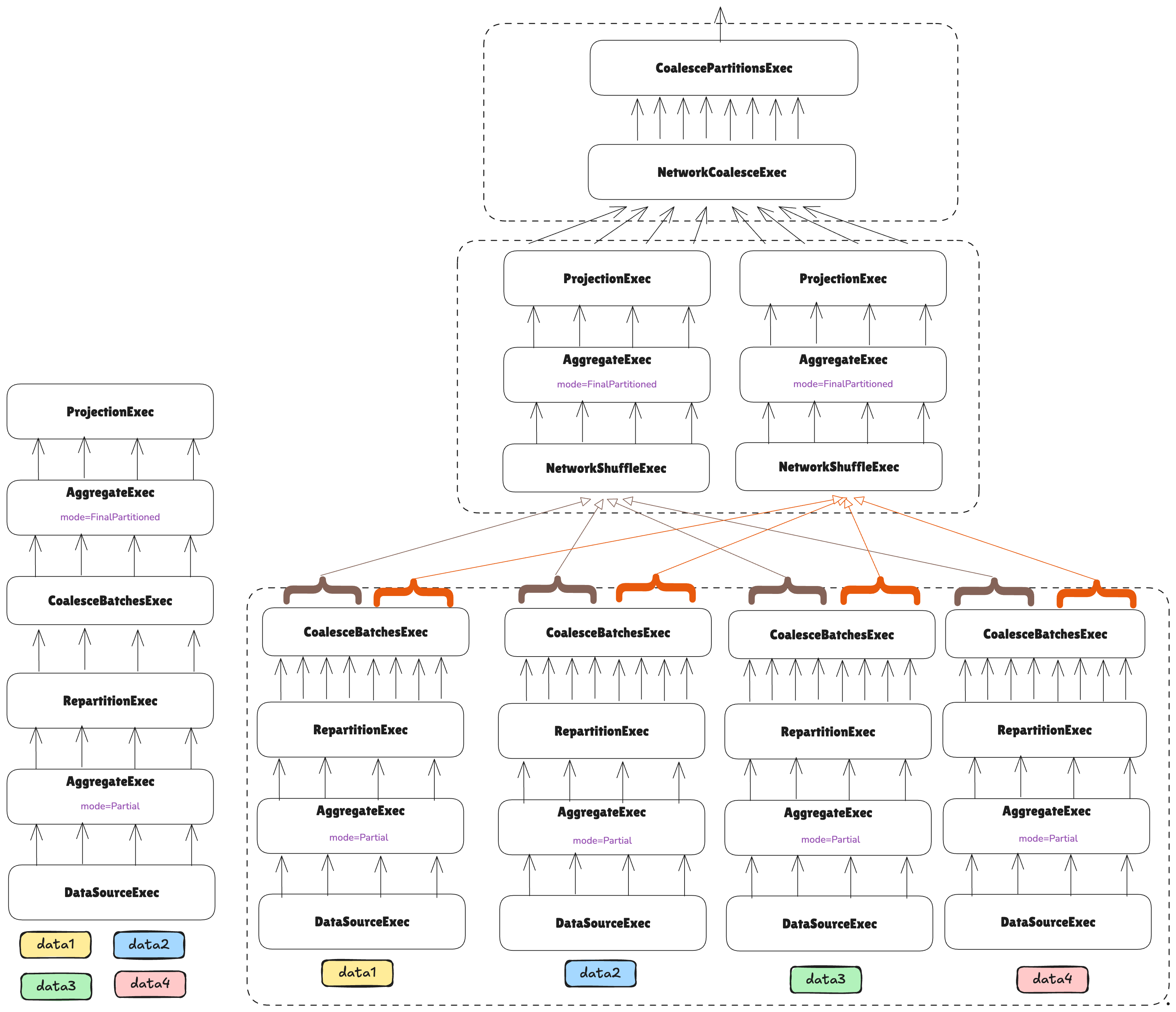
Note how at this point, what the user sees is just an ExecutionPlan that can be executed as any other normal plan, but it will happen to be distributed under the hood.

How a Distributed Plan is Built#

The same plan, before and after#

Reading the output#

Step by step#

This Page