Optimizing Distributed Joins, Sorts, and Aggregates with Dynamic Filtering

September 20, 2026 · Jayant Shrivastava (@jayshrivastava)

DataFusion implements an optimization called dynamic filtering, which applies runtime filters generated during execution. Dynamic filtering relies on shared memory to propagate updates from filter producers to consumers, which means that it does not automatically work in a distributed environment. This blog post will cover how we implemented this important optimization in DataFusion-Distributed.

Background and Motivation

Consider a join between a small dim table and a large fact table:

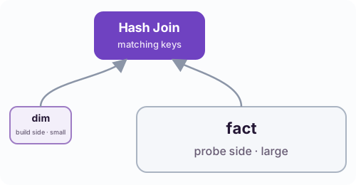
A hash join first reads the small input, called the build side, and creates a hash table from its join keys. It then reads the large probe side and looks up each probe key in that table.

Without dynamic filtering, the probe side performs work for rows that the join will ultimately discard:

• decoding files

• materializing columnar buffers

• hashing join columns

• evaluating expressions

• executing any potential operators between the scan and join

With dynamic filtering, the join’s hash table can be pushed down to the data source via shared memory, filtering out rows earlier to avoid wasted work:

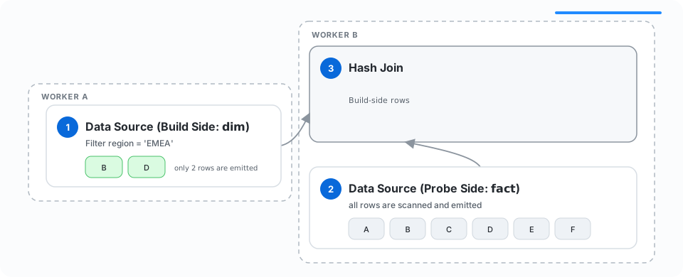
Figure 1

In Figure 1, the producer of the runtime filter, the hash join, is collocated on the same worker with the probe-side scan, so the runtime filter can be propagated via shared memory.

Notably, the collocated case relies on shared references being preserved after protobuf serialization, an important feature unblocked by #21807 and #22011, building upon prior work by Adrian Garcia Badaracco in #15566 and #15568.

For the non-collocated case (i.e., the “remote” case), we cannot rely on the standard mechanism:

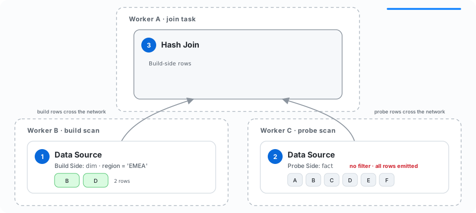
Figure 2

Figure 2 shows a scenario where dynamic filtering does not work out of the box, meaning extra work, such as serialization overhead and network transfer, is incurred.

In addition to hash joins, other operators like sorts and aggregates may publish runtime filters/bounds to push down. In this post, we describe how DataFusion-Distributed collects and carries these filters across process and network boundaries and evaluates performance using TPC-DS as a benchmark.

Design

There are two main problems to solve:

1. Correctness: Producers may be partitioned across different workers and produce distinct expressions. What filters do we propagate to consumers? How do we ensure we prune the correct rows?

2. Routing: Consumers may be partitioned across workers and be partitioned differently than the producers. How do we route filters from producers to consumers?

The answer to these problems, implemented in DataFusion-Distributed, is similar to the approach taken by Trino and Spark:

1. Planning: Discover producer-consumer relationships

2. Collecting and Merging: Get filter expressions from producers and merge them

3. Forwarding and Applying: Propagate merged expressions to consumers

1. Planning

Planning happens on a single query coordinator node. A plan tree is split vertically into stage boundaries and each stage is split horizontally into parallel tasks. The example below has two producer stages and one consumer stage consuming both filters:

┌─ Stage 3 · 2 tasks
│ HashJoinExec producers=[1]
│   ...
│   NetworkShuffleExec
└────────────────────────────
  ┌─ Stage 2 · 4 tasks
  │ HashJoinExec producers=[2]
  │   ...
  │   NetworkShuffleExec
  └──────────────────────────
    ┌─ Stage 1 · 8 tasks
    │   ...
    │ DataSourceExec consumers=[1, 2]
    └──────────────────────────────

At planning time, producer-consumer relationships are discovered using DataFusion-native APIs:

• PhysicalExpr::expression_id() uniquely identifies the same logical filter among plan nodes (#21807).

• ExecutionPlan::apply_expressions() finds expressions owned by consumers (#24018), building on work by Lía Castañeda in #20337.

• ExecutionPlan::dynamic_expressions_produced() identifies dynamic filter producers (#24068).

2. Collecting and Merging

Consider a partitioned producer that produces distinct filters F1, …, Fn. The safest option is to OR them together, permitting a row accepted by any producer from 1 through n. This preserves correctness at the cost of lower selectivity due to the OR removing partition-specific filtering.

From that safe default, we can implement tighter bounds based on the expression or producer type, as summarized below.

Producer shape	Wait for All Producers?	Continuous Forwarding?	Merge Behavior
Partitioned hash join	Yes	No, forward once	F0 OR F1 OR … OR Fn Safest default
CollectLeft hash join	No	No, forward once	Forward Ffirst
MIN/MAX aggregate	No	Yes, forward all updates	F0 AND F1 AND … AND Fn
TopK sort	No	Yes, forward all updates	F0 AND F1 AND … AND Fn

Table 1

CollectLeft Hash Join

CollectLeft broadcasts one complete build side to every join task. After a task finishes building its hash table, its predicate is equivalent to every other task’s predicate. The coordinator can therefore forward the first complete filter to all consumers instead of waiting for duplicate reports.

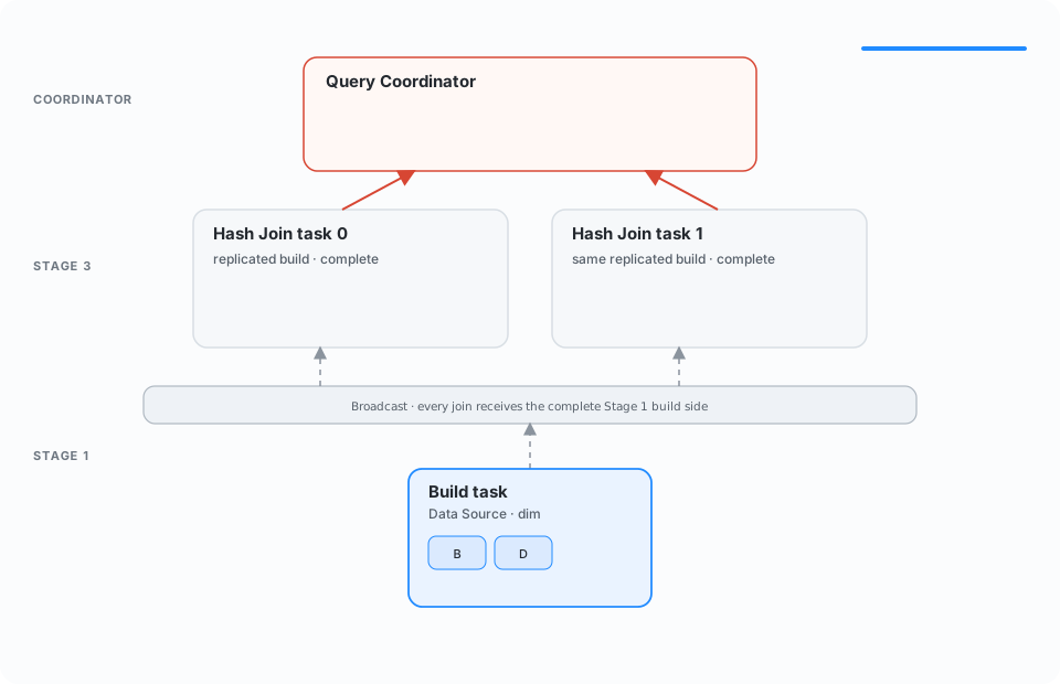
Figure 3

Partitioned Hash Join

Each partitioned join task sees only one slice of the build side. Publishing Fi alone could reject a key owned by task j where i != j. So, the coordinator waits for all build tasks to publish complete filter expressions and unions them together: Fglobal = F0 OR F1 OR ... OR Fn. Every matching consumer receives that safe global predicate.

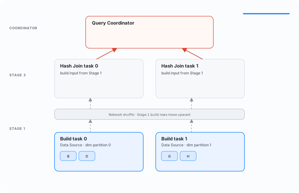
Figure 4

A Note on CASE hash(expr)

Each filter-producing task can itself contain multiple hash partitions, controlled by target_partitions. With target_partitions=4, a task’s expression looks like this:

CASE hash(row) % 4
  WHEN 0 THEN F0_P0(row)
  WHEN 1 THEN F0_P1(row)
  WHEN 2 THEN F0_P2(row)
  WHEN 3 THEN F0_P3(row)
END

Two tasks therefore create eight effective partitions, currently represented by OR-ing two per-task expressions:

CASE hash(row) % 4
  WHEN 0 THEN F0_P0(row)
  WHEN 1 THEN F0_P1(row)
  WHEN 2 THEN F0_P2(row)
  WHEN 3 THEN F0_P3(row)
END

OR

CASE hash(row) % 4
  WHEN 0 THEN F1_P0(row)
  WHEN 1 THEN F1_P1(row)
  WHEN 2 THEN F1_P2(row)
  WHEN 3 THEN F1_P3(row)
END

This is correct because:

(hash(key) % M) % N = hash(key) % N, when M is a multiple of N

In the running example, M=8 is the number of effective partitions across 2 tasks, and N=4 is the number of partitions per task. Consider a row routed to global partition 5. It must select partition 1 in each CASE expression for correctness. The tradeoff is reduced selectivity: 8 effective partitions behave like 4. ORing means we may admit extra rows, but it also means we cannot reject a valid row.

A more selective alternative is one large expression keyed by the global partition index:

CASE hash(row) % 8
  WHEN 0 THEN F0_P0(row)
  ...
  WHEN 4 THEN F1_P0(row)
  ...
  WHEN 7 THEN F1_P3(row)
END

The global CASE preserves selectivity by preserving all eight partitions, but it tightly couples DataFusion-Distributed to the underlying CASE expressions, which may change in the future. It can also create hundreds of CASE branches whose evaluation cost could counteract the benefits of early pruning. The simpler global OR is therefore the current default. Improving selectivity remains potential future work as upstream expression evaluation improves.

MIN/MAX Aggregate

Partial aggregates computing scalar MIN or MAX values can publish bounds that reject rows unable to improve the result. Each published bound is independently safe, so the coordinator intersects updates with AND and forwards successively tighter predicates without waiting for all producers.

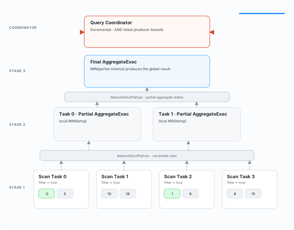
Figure 5

TopK Sort

A distributed TopK consists of per-task sorts followed by a SortPreservingMerge that produces the global result. Each task’s current Kth-value bound is independently safe. The coordinator intersects those bounds with AND and sends useful generations to remote scans while the merge continues.

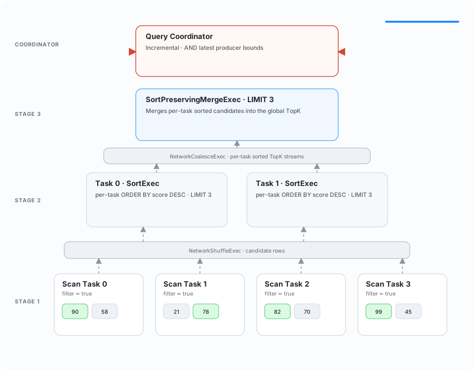
Figure 6

3. Forwarding and Applying

Once a safe predicate is ready, the coordinator sends it to workers that contain at least one consumer with the matching expression_id, which are already known from planning. Workers apply these expressions to their local running plans.

Consumers do not necessarily wait for remote filters. With sorts and aggregates, the scan often starts before the filter arrives. With joins, the probe side is naturally not polled until the build side is ready.

Benchmarks

We benchmarked the implementation using TPC-DS at scale_factor=10 in two scenarios:

• Local: one 16-core ARM host with 61.4 GiB of memory, four local gRPC workers with target_partitions=4 per worker, and local instance storage.

• Distributed: 12 c5n.4xlarge nodes, 15 CPUs and target_partitions=15 per worker, and data on S3.

Local Benchmark Results

Figure 7 shows the ten largest local improvements.

parquet={on,off} refers to the following DataFusion configuration options:

• datafusion.execution.parquet.pushdown_filters: evaluates predicates during Parquet decoding

• datafusion.execution.parquet.reorder_filters: heuristically reorders pushed-down predicates to reduce evaluation cost

The average speedup across the full TPC-DS suite was 1.05x with parquet=off and 1.20x with parquet=on.

With parquet=on, a dynamic predicate can participate in row-group, page-level, and decoder-level row pruning, which evidently is more valuable than pruning rows after the fact. The upstream DataFusion dynamic-filtering results similarly show the importance of scan-level pruning when using dynamic filtering.

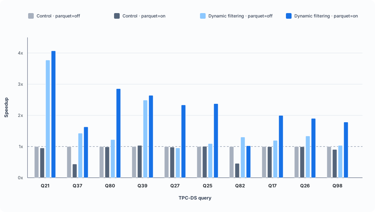
Figure 7

Q80 shows a clear improvement via metrics:

Metric	Dynamic filtering off	Dynamic filtering on
Speedup	1.00x	2.72x
Scan output rows, summed	55.47 million	6.23 million
Join input rows, summed	108.19 million	9.68 million
Network transfer	1.02 GB	88.1 MB
Join compute, summed	4,122 ms	609 ms
Coordinator updates received	0	80.3

Table 2

Latency improved 2.72x, and more than 90% of network traffic disappeared before the joins and shuffles.

Despite an average improvement of 1.20x with parquet=on, the optimization is still not a consistent win. Figure 8 shows the ten largest regressions:

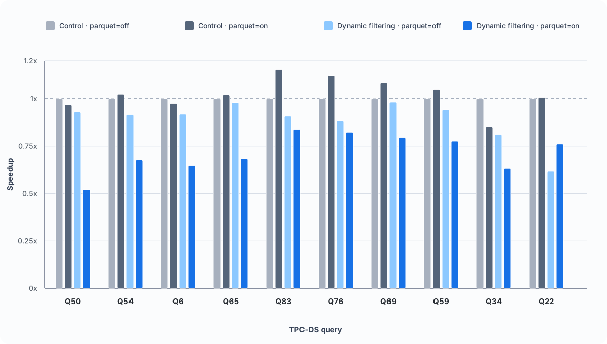
Figure 8

Q50 explains the regressions. A remote partitioned join sends a predicate to the large store_sales table, but the predicate is broad and expensive to evaluate:

Metric	Dynamic filtering off	Dynamic filtering on
Speedup	1.00x	0.54x
store_sales predicate evaluation	~0 s	4.61 s
store_sales output rows	28.80 million	26.70 million
store_sales bytes scanned	168.67 MB	171.72 MB
Total join compute	1.75 s	1.69 s

Table 3

The scan spends 4.61 seconds of summed task time evaluating the predicate, but eliminates only 7% of sales rows and saves no scan bytes. The join compute time is basically unchanged and does not repay that filter evaluation cost.

Distributed Benchmark Results

In the distributed scenario, we re-ran the ten queries that demonstrated the best local improvement. The results are summarized in Figure 9.

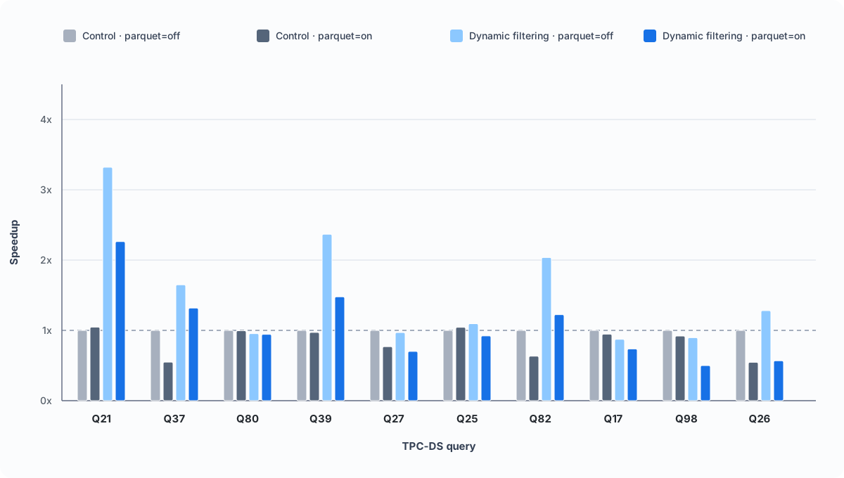
Figure 9

Only five queries reproduced a performance gain (in any parquet configuration).

We investigated Q80 to see why. Despite the higher network latency in a non-local scenario, dynamic filters arrived on time and pruned the same number of rows. The main difference was in the scan behavior.

Metric	Dynamic filtering off	Dynamic filtering on
Execution speedup	1.00x	0.855x
First-result latency	803 ms	943 ms
Critical store_sales output	28.800 M rows	0.592 M rows
Decoder data requested	1.058 GB	1.058 GB
Decoder reads per output stream	1	5
Mean file-stream first-batch delay	151 ms	339 ms
Critical fact-stage finish	771 ms	906 ms
Total network transfer	1.353 GB	128 MB
Critical scan-poll CPU, summed	2.801 s	2.432 s

Table 4

Q80 removes 98% of critical scan rows and 91% of network traffic, yet the query regresses. Scan CPU falls 13%, ruling out expensive predicate evaluation as the cause. Figure 10 shows the actual reason for the increased latency.

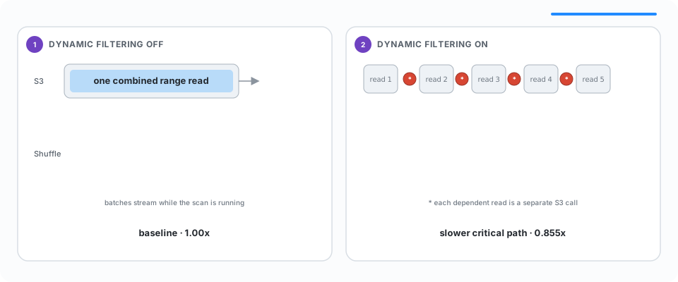
Figure 10

Without dynamic filtering, one combined S3 range read is used per file. With filtering, the Parquet data source issues five dependent reads. Each red marker in Figure 10 represents a separate S3 call. Five synchronous I/O operations are cheap against warm local storage, but expensive when the data needs to be downloaded. This overhead turns Q80’s local 2.72x improvement into a 0.855x regression in a distributed setting. Fortunately, DataFusion issue #24393 tracks this exact problem, and DataFusion makes it easy to implement a custom data source that does not use this I/O pattern.

Conclusion

Distributed dynamic filtering is implemented with DataFusion’s native physical plan and expression APIs. Colocated filters are automatically propagated to consumers via shared memory, while remote filters require merging and forwarding via the coordinator.

For dynamic filtering to be effective, it is important to consider the following:

1. Dynamic filtering is most valuable when it prevents rows from being read and decoded. Pushing down to the decoder level or remote data sources will yield the best results.

2. Dynamic filtering is a tradeoff. It wins when early pruning saves more work than the filter propagation and predicate evaluation cost.

3. Connector and leaf-node implementations matter. Access patterns and predicate pushdown can make or break the optimization.

Special thanks to Andrew Lamb (@alamb), Adrian Garcia Badaracco (@adriangb), Lía Castañeda (@LiaCastaneda), Gabriel Musat Mestre (@GabrielMusat), Gene Bordegaray (@gene-bordegaray), and the Apache DataFusion community for their design, implementation, and review work.